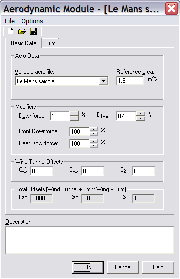
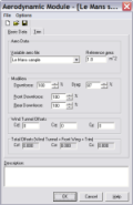
Aerodynamics
Aerodynamic values can be fixed or fully ride height dependent,
taken from an aero map file of lift, drag and balance as tabulated
functions of front and rear ride height.
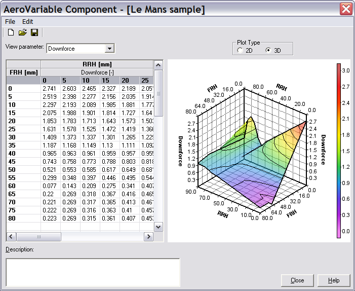
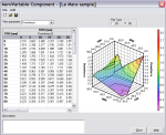
AeroContour will create correctly
formatted aero maps from arbitrary, scattered data aero data points.
This map can include front wing performance - the front wing
angle can be entered directly and the resulting change to overall
aero values automatically calculated.
The aeromap can be viewed as a 2D or 3D contour plot. In 3D mode
you can spin it with the mouse to see its shape.
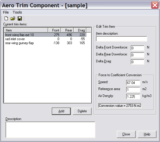
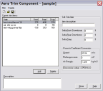
The aero trim can also be changed by selecting named items from a
user-defined trim file. These features make changes to the
aerodynamic setup very quick for race engineers, without the need to
look for extra data in other places.
Separate wind tunnel offsets can be entered to correct for wind
tunnel-track differences. For what-if studies and simulation
adjustment the frontal area can be changed and lift and drag values
scaled independently from the reference values.
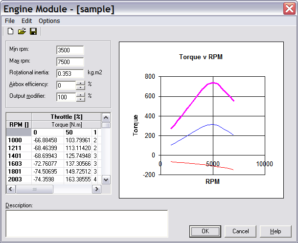
Engine
The engine model uses a graph of steady state output which can be
entered as either torque or power. Multiple curves can be entered
for different throttle openings, with negative values at low or zero
throttle. Optionally you can define a different engine map for each
gear. You can also optionally define different engine maps to be
used at different positions on the track giving very fine levels of
control over engine behaviour.
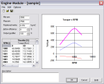
As with all tables in AeroLap a graph is plotted as you
enter values, making it easy to see the effect of changes. A rev
limit, minimum allowed revs and engine rotational inertia can also
be defined, as can the engine's fuel consumption.
You can scale the power output linearly up or down to see the
effect of gross changes to engine performance, and model the effect
of airbox efficiency on ram air pressure. The engine model
automatically accounts for atmospheric pressure defined by the
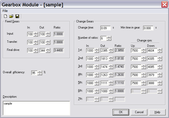
Environment module. Gearbox
The gearbox can have any number of
change gears up to seven, plus input, transfer and final drive
gears.
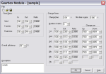
Each change ratio has separate change up and change down rpm values
to control driver behaviour. Gears can also be set according to
track position e.g. you can force a gear choice at a corner. You can
also specify the minimum time to hold a gear, and the gear change
time. A "lazy" gear change strategy can be enabled, which holds high
gears as long as possible. The overall
transmission efficiency can be defined. Track
The track can be created in two ways:
-
Automatically from data you have already acquired on most
major data acquisition systems;
-
Manually by entering multiple straight and curved elements -
useful when simulating tracks you have no data for.
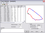
Tracks can be made from any number of straight or curved
elements, from a couple to thousands giving highly realistic
representation. Each element has its own bank angle, gradient,
vertical radius (crests and dips) and local grip factor
so you can model sticky or slippery spots. You can force gear
selection on particular sections of track. Graphical highlighting of
selected track elements on the track map make quick local property
modifications easy. A track profile editor makes it straightforward
to define banking and gradient around the track.
|
Chassis
The chassis model defines the masses and
dimensions of the car. The car may be setup symmetrically or
asymmetrically, with values entered for each corner. Values can be
given for the car in a setup condition, e.g. on setup wheels or
without a driver, and then automatically modified to the race
condition by entering offsets.
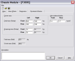
Fuel volume can be varied from the reference value and new static
mass, distribution and ride heights automatically calculated.
Driver behaviour can be altered, with braking and throttle pedal
application rates. Brake proportioning can be fixed or ABS. The
drivetrain can be FWD, RWD or 4WD.
Suspension
The suspension is modelled with anti-squat and dive angles; roll
centre effects; static ride heights; bump and droop travel; spring
and anti-roll bar stiffness and preload. Centre springs can be used.
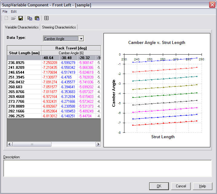
Most properties can be entered as fixed values, or as 2D tables varying
with damper deflection and rack travel.
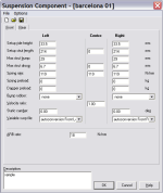
These 2D tables can be generated from a set of suspension joint
positions by AeroSusp, a separately
available 3D suspension
kinematics program.

You can define non-linear, asymmetric steering characteristics,
with bump steer and Ackerman effects.
The vertical installation stiffness and camber and toe compliance
of the suspension may also be defined.
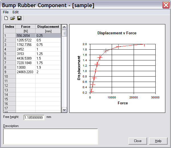
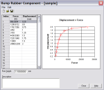
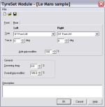
Non-linear bump rubber characteristics can be used. Once defined,
variable characteristics or bump rubbers may easily be chosen from
drop down lists of existing components.
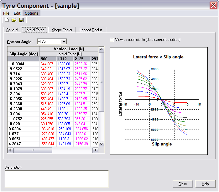
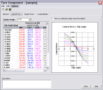
Tires
Tire grip characteristics are entered as a table of slip angle
against lateral force and camber for multiple loads and camber
angles. Only one load and camber must be provided if you don't have
comprehensive data. The smallest amount of data to define a working
tire is around 6 numbers. Fully detailed tires can use thousands of
values. If Pacejka/MF-Tyre model coefficients are available, the
tables can be automatically generated from the coefficients.
Combined grip is modelled with a variable aspect ratio friction
ellipse that is a function of vertical load and camber. Load
sensitivity is handled with a load dependent friction coefficient
drop-off for out of range values, otherwise supplied values are
used. Overall tire grip can be scaled up and down. You can also set
local grip values in the track editor.
Tire stiffness and loaded radius data are used for overall
vehicle load transfer and ride height calculations. Dynamic loaded
radius can be modelled as a non-linear function of speed, camber and
vertical load. Toe-in can be set front and rear.
Grip can be varied per axle or globally, as well as by track
position.
Environment
A prevailing wind can be added to the simulation with a speed and
direction. You can also set a different wind speed and
direction for every element that makes up the track, if you want to
model a variable wind field.
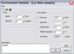
Air density is calculated for you with inputs of humidity,
temperature and pressure. This affects both aerodynamic and engine
performance. If you are modelling an event you don't have pressure
data for, for example a race coming up, then you can specify
altitude instead and pressure will be found from a standard
atmosphere model. |